SEAI 2021 - Python - Lab 1
Intro to Python
Vincenzo Nardelli - vincnardelli@gmail.com - https://github.com/vincnardelli
Lab structure:
- Intro
- 1 - Matrix computation with NumPy
- 2 - Data manipulation and analysis with Pandas
- 3 - Graphs with Matplotlib and Seaborn
- Extra topic: Git and Github (with Niccolò Salvini)
Let’s start from the basics!
3 + 5
8
12 / 7
1.7142857142857142
result = 3 + 5
result
8
print(result)
8
result = result * 3.1415
print(result)
25.132
vector = [1, 3, 8, 13]
vector * 3
[1, 3, 8, 13, 1, 3, 8, 13, 1, 3, 8, 13]
dict = {'a': 12,
        'b': 34,
        'c': 62,
        'd': 68,
        'e': 29}
dict
{'a': 12, 'b': 34, 'c': 62, 'd': 68, 'e': 29}
Unlike R, the basic version of Python does not allow operations between scalars and matrices. For this you need to convert the vector to numpy array.
The package functions must be called taking into account the library structure
import numpy as np
vector = np.array(vector)
vector
array([ 1, 3, 8, 13])
vector * 3
array([ 3, 9, 24, 39])
The procedure for the subset is similar to that of R but it must be taken into account that the numbering starts from 0 instead of 1.
vector[1]
3
vector[0]
1
Furthermore, in the case of multiple selection, the index starts from 0 (unlike R which starts from 1) and the second value representing the last element is NOT included in the subset (unlike R which is included).
vector[1:3]
array([3, 8])
vector[[False, True, True, False]]
array([3, 8])
vector < 3
array([ True, False, False, False])
vector[vector < 3]
array([1])
L = list(range(10))
L
[0, 1, 2, 3, 4, 5, 6, 7, 8, 9]
type(L[0])
int
Or, similarly, a list of strings:
L2 = []
for c in L:
    L2.append(str(c))
print(L2)
['0', '1', '2', '3', '4', '5', '6', '7', '8', '9']
L2 = [str(c) for c in L]
L2
['0', '1', '2', '3', '4', '5', '6', '7', '8', '9']
type(L2[0])
str
Because of Python’s dynamic typing, we can even create heterogeneous lists:
L3 = [True, "2", 3.0, 4]
[type(item) for item in L3]
[bool, str, float, int]
1 - Matrix computation with NumPy
- Creating arrays from Python listis
- Creating arrays from Scratch
- NumPy Standard Data Types
- Array Attributes
- Array Indexing
- Array Slicing
- Arithmetic Operations
NumPy brings the computational power of languages like C and Fortran to Python!
Why use NumPy? It’s fast
-
In a Python object, to allow the flexible types, each item in the list must contain its own type info, reference count, and other information.
-
In a computational task we are in the special case that all variables are of the same type, much of this information is redundant: it can be much more efficient to store data in a fixed-type array.
The difference between a dynamic-type list and a fixed-type (NumPy-style) array is illustrated in the following figure:
At the implementation level, the array essentially contains a single pointer to one contiguous block of data.
The Python list, on the other hand, contains a pointer to a block of pointers, each of which in turn points to a full Python object.
Again, the advantage of the list is flexibility: because each list element is a full structure containing both data and type information, the list can be filled with data of any desired type. Fixed-type NumPy-style arrays lack this flexibility, but are much more efficient for storing and manipulating data.
import numpy as np
Creating Arrays from Python Lists
# integer array:
np.array([1, 4, 2, 5, 3])
array([1, 4, 2, 5, 3])
np.array([3.14, 4, 2, 3])
array([3.14, 4. , 2. , 3. ])
np.array([1, 2, 3, 4], dtype='float32')
array([1., 2., 3., 4.], dtype=float32)
# nested lists result in multi-dimensional arrays
np.array([range(i, i + 3) for i in [2, 4, 6]])
array([[2, 3, 4],
       [4, 5, 6],
       [6, 7, 8]])
Creating Arrays from Scratch
Create a length-10 integer array filled with zeros
np.zeros(10, dtype=int)
array([0, 0, 0, 0, 0, 0, 0, 0, 0, 0])
Create a 3x5 floating-point array filled with ones
np.ones((3, 5), dtype=float)
array([[1., 1., 1., 1., 1.],
       [1., 1., 1., 1., 1.],
       [1., 1., 1., 1., 1.]])
Create an array filled with a linear sequence Starting at 0, ending at 20, stepping by 2
np.arange(0, 20, 2)
array([ 0, 2, 4, 6, 8, 10, 12, 14, 16, 18])
Create an array of five values evenly spaced between 0 and 1
np.linspace(0, 1, 5)
array([0. , 0.25, 0.5 , 0.75, 1. ])
Create a 3x3 array of normally distributed random values with mean 0 and standard deviation 1
np.random.normal(0, 1, (3, 3))
array([[-1.02677226,  1.11060734,  0.03739026],
       [-0.24285475,  0.88068307,  0.94551808],
       [-0.06911716, -0.09423746, -1.25280425]])
Create a 3x3 identity matrix
np.eye(3)
array([[1., 0., 0.],
       [0., 1., 0.],
       [0., 0., 1.]])
NumPy Standard Data Types
Because NumPy is built in C, the types will be familiar to users of C, Fortran, and other related languages.
np.zeros(10, dtype=np.int16)
array([0, 0, 0, 0, 0, 0, 0, 0, 0, 0], dtype=int16)
| Data type | Description |
|---|---|
bool_ |
Boolean (True or False) stored as a byte |
int_ |
Default integer type (same as C long; normally either int64 or int32) |
intc |
Identical to C int (normally int32 or int64) |
intp |
Integer used for indexing (same as C ssize_t; normally either int32 or int64) |
int8 |
Byte (-128 to 127) |
int16 |
Integer (-32768 to 32767) |
int32 |
Integer (-2147483648 to 2147483647) |
int64 |
Integer (-9223372036854775808 to 9223372036854775807) |
uint8 |
Unsigned integer (0 to 255) |
uint16 |
Unsigned integer (0 to 65535) |
uint32 |
Unsigned integer (0 to 4294967295) |
uint64 |
Unsigned integer (0 to 18446744073709551615) |
float_ |
Shorthand for float64. |
float16 |
Half precision float: sign bit, 5 bits exponent, 10 bits mantissa |
float32 |
Single precision float: sign bit, 8 bits exponent, 23 bits mantissa |
float64 |
Double precision float: sign bit, 11 bits exponent, 52 bits mantissa |
complex_ |
Shorthand for complex128. |
complex64 |
Complex number, represented by two 32-bit floats |
complex128 |
Complex number, represented by two 64-bit floats |
Array Attributes
One-dimensional array
np.random.seed(0)

x1 = np.random.randint(10, size=6)
x1
array([5, 0, 3, 3, 7, 9])
Two-dimensional array
x2 = np.random.randint(10, size=(3, 4))
x2
array([[3, 5, 2, 4],
       [7, 6, 8, 8],
       [1, 6, 7, 7]])
Three-dimensional array
x3 = np.random.randint(10, size=(3, 4, 5))  # Three-dimensional array
x3
array([[[8, 1, 5, 9, 8],
        [9, 4, 3, 0, 3],
        [5, 0, 2, 3, 8],
        [1, 3, 3, 3, 7]],

       [[0, 1, 9, 9, 0],
        [4, 7, 3, 2, 7],
        [2, 0, 0, 4, 5],
        [5, 6, 8, 4, 1]],

       [[4, 9, 8, 1, 1],
        [7, 9, 9, 3, 6],
        [7, 2, 0, 3, 5],
        [9, 4, 4, 6, 4]]])
Each array has attributes ndim (the number of dimensions), shape (the size of each dimension), and size (the total size of the array):
print("x3 ndim: ", x3.ndim)
print("x3 shape:", x3.shape)
print("x3 size: ", x3.size)
x3 ndim:  3
x3 shape: (3, 4, 5)
x3 size:  60
Another useful attribute is the dtype, the data type of the array (which we discussed previously in Understanding Data Types in Python):
print("dtype:", x3.dtype)
dtype: int64
Array Indexing
In a one-dimensional array, the $i^{th}$ value (counting from zero) can be accessed by specifying the desired index in square brackets, just as with Python lists:
x1
array([5, 0, 3, 3, 7, 9])
x1[0]
5
x1[4]
7
To index from the end of the array, you can use negative indices:
x1[-1]
9
x1[-2]
7
In a multi-dimensional array, items can be accessed using a comma-separated tuple of indices:
x2
array([[3, 5, 2, 4],
       [7, 6, 8, 8],
       [1, 6, 7, 7]])
x2[0, 0]
3
x2[2, 0]
1
x2[2, -1]
7
Values can also be modified using any of the above index notation:
x2[0, 0] = 12
x2
array([[12,  5,  2,  4],
       [ 7,  6,  8,  8],
       [ 1,  6,  7,  7]])
x1[0] = 3.14159  # this will be truncated!
x1
array([3, 0, 3, 3, 7, 9])
Array Slicing
Just as we can use square brackets to access individual array elements, we can also use them to access subarrays with the slice notation, marked by the colon (:) character.
The NumPy slicing syntax follows that of the standard Python list; to access a slice of an array x, use this:
x[start:stop:step]
If any of these are unspecified, they default to the values start=0, stop=size of dimension, step=1.
We’ll take a look at accessing sub-arrays in one dimension and in multiple dimensions.
x = np.arange(10)
x
array([0, 1, 2, 3, 4, 5, 6, 7, 8, 9])
First five element
x[:5]
array([0, 1, 2, 3, 4])
Elements after index 5
x[5:]
array([5, 6, 7, 8, 9])
middle sub-array
x[4:7]
array([4, 5, 6])
every other element
x[::2]
array([0, 2, 4, 6, 8])
every other element, starting at index 1
x[1::2]
array([1, 3, 5, 7, 9])
A potentially confusing case is when the step value is negative.
In this case, the defaults for start and stop are swapped.
This becomes a convenient way to reverse an array:
x[::-1] # all elements, reversed
array([9, 8, 7, 6, 5, 4, 3, 2, 1, 0])
x2
array([[12,  5,  2,  4],
       [ 7,  6,  8,  8],
       [ 1,  6,  7,  7]])
x2[:2, :3] # two rows, three columns
array([[12,  5,  2],
       [ 7,  6,  8]])
x2[:3, ::2] # all rows, every other column
array([[12,  2],
       [ 7,  8],
       [ 1,  7]])
Finally, subarray dimensions can even be reversed together:
x2[::-1, ::-1]
array([[ 7,  7,  6,  1],
       [ 8,  8,  6,  7],
       [ 4,  2,  5, 12]])
Accessing array rows and columns
One commonly needed routine is accessing of single rows or columns of an array.
This can be done by combining indexing and slicing, using an empty slice marked by a single colon (:):
print(x2[:, 0]) # first column of x2
[12 7 1]
print(x2[0, :]) # first row of x2
[12 5 2 4]
Arithmetic Operations
a = np.array([1,2,3])
b = np.array([(1.5,2,3), (4,5,6)], dtype = float)
a + b
array([[2.5, 4. , 6. ],
       [5. , 7. , 9. ]])
a - b
array([[-0.5,  0. ,  0. ],
       [-3. , -3. , -3. ]])
a * b
array([[ 1.5,  4. ,  9. ],
       [ 4. , 10. , 18. ]])
a / b
array([[0.66666667, 1.        , 1.        ],
       [0.25      , 0.4       , 0.5       ]])
np.exp(a)
array([ 2.71828183, 7.3890561 , 20.08553692])
np.log(a)
array([0. , 0.69314718, 1.09861229])
c = np.array([1.5,2], dtype = float)
c
array([1.5, 2. ])
d = np.array([4,5], dtype = float)
d
array([4., 5.])
c.dot(d)
16.0
1.5*4+2*5
16.0
2 - Data manipulation and analysis with Pandas
Pandas is a Python data analysis Library. The name is derived from the term “panel data”.
- The Pandas Series Object
- The Pandas DataFrame Object
- Construction DataFrame Objects
- Data loading
- Data indexing and selection
- Aggregation and grouping
- Simple aggregation
- GroupBy
- Aggregate, filter and transform
import pandas as pd
#pd.DataFrame?
The Pandas Series Object
A Pandas Series is a one-dimensional array of indexed data.
It can be created from a list or array as follows:
data = pd.Series([0.25, 0.5, 0.75, 1.0])
data
0    0.25
1    0.50
2    0.75
3    1.00
dtype: float64
As we see in the output, the Series wraps both a sequence of values and a sequence of indices, which we can access with the values and index attributes.
The values are simply a familiar NumPy array:
data.values
array([0.25, 0.5 , 0.75, 1. ])
The index is an array-like object of type pd.Index, which we’ll discuss in more detail momentarily.
data.index
RangeIndex(start=0, stop=4, step=1)
Like with a NumPy array, data can be accessed by the associated index via the familiar Python square-bracket notation:
data[1]
0.5
data[1:3]
1    0.50
2    0.75
dtype: float64
population_dict = {'California': 38332521,
                   'Texas': 26448193,
                   'New York': 19651127,
                   'Florida': 19552860,
                   'Illinois': 12882135}
population = pd.Series(population_dict)
population
California    38332521
Texas         26448193
New York      19651127
Florida       19552860
Illinois      12882135
dtype: int64
By default, a Series will be created where the index is drawn from the sorted keys.
From here, typical dictionary-style item access can be performed:
population['California']
38332521
Unlike a dictionary, though, the Series also supports array-style operations such as slicing:
population['New York':'Illinois']
New York    19651127
Florida     19552860
Illinois    12882135
dtype: int64
population[2:5]
New York    19651127
Florida     19552860
Illinois    12882135
dtype: int64
The Pandas DataFrame Object
The next fundamental structure in Pandas is the DataFrame.
The DataFrame can be thought of either as a generalization of a NumPy array, or as a specialization of a Python dictionary.
DataFrame as a generalized NumPy array
A DataFrame is an analog of a two-dimensional array with both flexible row indices and flexible column names.
Just as you might think of a two-dimensional array as an ordered sequence of aligned one-dimensional columns, you can think of a DataFrame as a sequence of aligned Series objects.
Here, by “aligned” we mean that they share the same index.
area_dict = {'California': 423967, 'Texas': 695662, 'New York': 141297,
             'Florida': 170312, 'Illinois': 149995}
area = pd.Series(area_dict)
area
California    423967
Texas         695662
New York      141297
Florida       170312
Illinois      149995
dtype: int64
states = pd.DataFrame({'population': population,
                       'area': area})
states
| population | area | |
|---|---|---|
| California | 38332521 | 423967 |
| Texas | 26448193 | 695662 |
| New York | 19651127 | 141297 |
| Florida | 19552860 | 170312 |
| Illinois | 12882135 | 149995 |
states.index
Index(['California', 'Texas', 'New York', 'Florida', 'Illinois'], dtype='object')
states.columns
Index(['population', 'area'], dtype='object')
Thus the DataFrame can be thought of as a generalization of a two-dimensional NumPy array, where both the rows and columns have a generalized index for accessing the data.
DataFrame as specialized dictionary
Similarly, we can also think of a DataFrame as a specialization of a dictionary.
Where a dictionary maps a key to a value, a DataFrame maps a column name to a Series of column data.
For example, asking for the 'area' attribute returns the Series object containing the areas we saw earlier:
states['area']
California    423967
Texas         695662
New York      141297
Florida       170312
Illinois      149995
Name: area, dtype: int64
Constructing DataFrame objects
From a single Series object
pd.DataFrame(population, columns=['population'])
| population | |
|---|---|
| California | 38332521 |
| Texas | 26448193 |
| New York | 19651127 |
| Florida | 19552860 |
| Illinois | 12882135 |
From a list of dicts
Any list of dictionaries can be made into a DataFrame.
data = [{'a': i, 'b': 2 * i}
        for i in range(3)]
pd.DataFrame(data)
| a | b | |
|---|---|---|
| 0 | 0 | 0 |
| 1 | 1 | 2 |
| 2 | 2 | 4 |
Even if some keys in the dictionary are missing, Pandas will fill them in with NaN (i.e., “not a number”) values:
pd.DataFrame([{'a': 1, 'b': 2}, {'b': 3, 'c': 4}])
| a | b | c | |
|---|---|---|---|
| 0 | 1.0 | 2 | NaN |
| 1 | NaN | 3 | 4.0 |
From a two-dimensional NumPy array
pd.DataFrame(np.random.rand(3, 2),
             columns=['foo', 'bar'],
             index=['a', 'b', 'c'])
| foo | bar | |
|---|---|---|
| a | 0.652790 | 0.635059 |
| b | 0.995300 | 0.581850 |
| c | 0.414369 | 0.474698 |
Data loading
path = "https://raw.githubusercontent.com/pandas-dev/pandas/master/doc/data/titanic.csv"
titanic = pd.read_csv(path)
titanic.head()
| PassengerId | Survived | Pclass | Name | Sex | Age | SibSp | Parch | Ticket | Fare | Cabin | Embarked | |
|---|---|---|---|---|---|---|---|---|---|---|---|---|
| 0 | 1 | 0 | 3 | Braund, Mr. Owen Harris | male | 22.0 | 1 | 0 | A/5 21171 | 7.2500 | NaN | S |
| 1 | 2 | 1 | 1 | Cumings, Mrs. John Bradley (Florence Briggs Th... | female | 38.0 | 1 | 0 | PC 17599 | 71.2833 | C85 | C |
| 2 | 3 | 1 | 3 | Heikkinen, Miss. Laina | female | 26.0 | 0 | 0 | STON/O2. 3101282 | 7.9250 | NaN | S |
| 3 | 4 | 1 | 1 | Futrelle, Mrs. Jacques Heath (Lily May Peel) | female | 35.0 | 1 | 0 | 113803 | 53.1000 | C123 | S |
| 4 | 5 | 0 | 3 | Allen, Mr. William Henry | male | 35.0 | 0 | 0 | 373450 | 8.0500 | NaN | S |
path_xls = "https://github.com/pandas-dev/pandas/blob/master/doc/data/test.xls?raw=true"
test = pd.read_excel(path_xls)
test
| Unnamed: 0 | A | B | C | D | |
|---|---|---|---|---|---|
| 0 | 2000-01-03 | 0.980269 | 3.685731 | -0.364217 | -1.159738 |
| 1 | 2000-01-04 | 1.047916 | -0.041232 | -0.161812 | 0.212549 |
| 2 | 2000-01-05 | 0.498581 | 0.731168 | -0.537677 | 1.346270 |
| 3 | 2000-01-06 | 1.120202 | 1.567621 | 0.003641 | 0.675253 |
| 4 | 2000-01-07 | -0.487094 | 0.571455 | -1.611639 | 0.103469 |
| 5 | 2000-01-10 | 0.836649 | 0.246462 | 0.588543 | 1.062782 |
| 6 | 2000-01-11 | -0.157161 | 1.340307 | 1.195778 | -1.097007 |
df = pd.read_html('https://en.wikipedia.org/wiki/List_of_largest_cities')[1]
df.head()
| City[a] | Country | Skyline | UN 2018 population estimates[b] | City proper[c] | Metropolitan area[d] | Urban area(Demographia)[12] | |||||
|---|---|---|---|---|---|---|---|---|---|---|---|
| City[a] | Country | Skyline | UN 2018 population estimates[b] | Definition | Population | Area(km2) | Population | Area(km2) | Population | Area(km2) | |
| 0 | Tokyo | Japan | NaN | 37400068 | Metropolis prefecture | 13,515,271[14] | 2,191[14] | 37,274,000[15] | 13,452[15] | 37977000.0 | 8,230[e] |
| 1 | Delhi | India | NaN | 28514000 | Capital City | 16,753,235[16] | 1484 | 29,000,000[17] | 3,483[17] | 29617000.0 | 2,232[f] |
| 2 | Shanghai | China | NaN | 25582000 | Municipality | 24,183,000[18] | 6341 | NaN | NaN | 22120000.0 | 4,068[g] |
| 3 | São Paulo | Brazil | NaN | 21650000 | Municipality | 12,252,023[19] | 1521 | 21,734,682[20] | 7947 | 22046000.0 | 3,116[h] |
| 4 | Mexico City | Mexico | NaN | 21581000 | City-state | 9,209,944[21] | 1485 | 21,804,515[21] | 7,866[22] | 20996000.0 | 2386 |
#df.to_csv("scraped_data.csv")
#df.to_excel("scraped_data.xlsx")
Data Indexing and Selection
states['area']
California    423967
Texas         695662
New York      141297
Florida       170312
Illinois      149995
Name: area, dtype: int64
Equivalently, we can use attribute-style access with column names that are strings:
states.area
California    423967
Texas         695662
New York      141297
Florida       170312
Illinois      149995
Name: area, dtype: int64
states['density'] = states['population'] / states['area']
states
| population | area | density | |
|---|---|---|---|
| California | 38332521 | 423967 | 90.413926 |
| Texas | 26448193 | 695662 | 38.018740 |
| New York | 19651127 | 141297 | 139.076746 |
| Florida | 19552860 | 170312 | 114.806121 |
| Illinois | 12882135 | 149995 | 85.883763 |
Thus for array-style indexing, we need another convention.
Here Pandas again uses the locand iloc indexers mentioned earlier.
Using the iloc indexer, we can index the underlying array as if it is a simple NumPy array (using the implicit Python-style index), but the DataFrame index and column labels are maintained in the result:
states.iloc[:3, :2]
| population | area | |
|---|---|---|
| California | 38332521 | 423967 |
| Texas | 26448193 | 695662 |
| New York | 19651127 | 141297 |
Similarly, using the loc indexer we can index the underlying data in an array-like style but using the explicit index and column names:
states.loc[:'New York', :'area']
| population | area | |
|---|---|---|
| California | 38332521 | 423967 |
| Texas | 26448193 | 695662 |
| New York | 19651127 | 141297 |
states.loc[states.density > 100, ['population', 'density']]
| population | density | |
|---|---|---|
| New York | 19651127 | 139.076746 |
| Florida | 19552860 | 114.806121 |
Additional indexing conventions
There are a couple extra indexing conventions that might seem at odds with the preceding discussion, but nevertheless can be very useful in practice. First, while indexing refers to columns, slicing refers to rows:
states['Florida':'Illinois']
| population | area | density | |
|---|---|---|---|
| Florida | 19552860 | 170312 | 114.806121 |
| Illinois | 12882135 | 149995 | 85.883763 |
Such slices can also refer to rows by number rather than by index:
states[1:3]
| population | area | density | |
|---|---|---|---|
| Texas | 26448193 | 695662 | 38.018740 |
| New York | 19651127 | 141297 | 139.076746 |
Similarly, direct masking operations are also interpreted row-wise rather than column-wise:
states[states.density > 100]
| population | area | density | |
|---|---|---|---|
| New York | 19651127 | 141297 | 139.076746 |
| Florida | 19552860 | 170312 | 114.806121 |
Aggregation and Grouping
An essential piece of analysis of large data is efficient summarization: computing aggregations like sum(), mean(), median(), min(), and max(), in which a single number gives insight into the nature of a potentially large dataset.
In this section, we’ll explore aggregations in Pandas, from simple operations akin to what we’ve seen on NumPy arrays, to more sophisticated operations based on the concept of a groupby.
Here we will use the Planets dataset, available via the Seaborn package (see Visualization With Seaborn). It gives information on planets that astronomers have discovered around other stars (known as extrasolar planets or exoplanets for short). It can be downloaded with a simple Seaborn command:
import seaborn as sns
planets = sns.load_dataset('planets')
planets.shape
(1035, 6)
planets.head()
| method | number | orbital_period | mass | distance | year | |
|---|---|---|---|---|---|---|
| 0 | Radial Velocity | 1 | 269.300 | 7.10 | 77.40 | 2006 |
| 1 | Radial Velocity | 1 | 874.774 | 2.21 | 56.95 | 2008 |
| 2 | Radial Velocity | 1 | 763.000 | 2.60 | 19.84 | 2011 |
| 3 | Radial Velocity | 1 | 326.030 | 19.40 | 110.62 | 2007 |
| 4 | Radial Velocity | 1 | 516.220 | 10.50 | 119.47 | 2009 |
This has some details on the 1,000+ extrasolar planets discovered up to 2014.
Simple Aggregation in Pandas
rng = np.random.RandomState(42)
ser = pd.Series(rng.rand(5))
ser
0    0.374540
1    0.950714
2    0.731994
3    0.598658
4    0.156019
dtype: float64
ser.sum()
2.811925491708157
ser.mean()
0.5623850983416314
For a DataFrame, by default the aggregates return results within each column:
df = pd.DataFrame({'A': rng.rand(5),
                   'B': rng.rand(5)})
df
| A | B | |
|---|---|---|
| 0 | 0.155995 | 0.020584 |
| 1 | 0.058084 | 0.969910 |
| 2 | 0.866176 | 0.832443 |
| 3 | 0.601115 | 0.212339 |
| 4 | 0.708073 | 0.181825 |
df.mean()
A    0.477888
B    0.443420
dtype: float64
By specifying the axis argument, you can instead aggregate within each row:
df.mean(axis='columns')
0    0.088290
1    0.513997
2    0.849309
3    0.406727
4    0.444949
dtype: float64
planets.dropna().describe()
| number | orbital_period | mass | distance | year | |
|---|---|---|---|---|---|
| count | 498.00000 | 498.000000 | 498.000000 | 498.000000 | 498.000000 |
| mean | 1.73494 | 835.778671 | 2.509320 | 52.068213 | 2007.377510 |
| std | 1.17572 | 1469.128259 | 3.636274 | 46.596041 | 4.167284 |
| min | 1.00000 | 1.328300 | 0.003600 | 1.350000 | 1989.000000 |
| 25% | 1.00000 | 38.272250 | 0.212500 | 24.497500 | 2005.000000 |
| 50% | 1.00000 | 357.000000 | 1.245000 | 39.940000 | 2009.000000 |
| 75% | 2.00000 | 999.600000 | 2.867500 | 59.332500 | 2011.000000 |
| max | 6.00000 | 17337.500000 | 25.000000 | 354.000000 | 2014.000000 |
The following table summarizes some other built-in Pandas aggregations:
| Aggregation | Description |
|---|---|
count() |
Total number of items |
first(), last() |
First and last item |
mean(), median() |
Mean and median |
min(), max() |
Minimum and maximum |
std(), var() |
Standard deviation and variance |
mad() |
Mean absolute deviation |
prod() |
Product of all items |
sum() |
Sum of all items |
These are all methods of DataFrame and Series objects.
GroupBy: Split, Apply, Combine
Simple aggregations can give you a flavor of your dataset, but often we would prefer to aggregate conditionally on some label or index: this is implemented in the so-called groupby operation.
The name “group by” comes from a command in the SQL database language, but it is perhaps more illuminative to think of it in the terms first coined by Hadley Wickham of Rstats fame: split, apply, combine.
A canonical example of this split-apply-combine operation, where the “apply” is a summation aggregation, is illustrated in this figure:
This makes clear what the groupby accomplishes:
- The split step involves breaking up and grouping a
DataFramedepending on the value of the specified key. - The apply step involves computing some function, usually an aggregate, transformation, or filtering, within the individual groups.
- The combine step merges the results of these operations into an output array.
df = pd.DataFrame({'key': ['A', 'B', 'C', 'A', 'B', 'C'],
                   'data': range(6)}, columns=['key', 'data'])
df
| key | data | |
|---|---|---|
| 0 | A | 0 |
| 1 | B | 1 |
| 2 | C | 2 |
| 3 | A | 3 |
| 4 | B | 4 |
| 5 | C | 5 |
df.groupby('key').sum()
| data | |
|---|---|
| key | |
| A | 3 |
| B | 5 |
| C | 7 |
The GroupBy object
planets.groupby('method')
<pandas.core.groupby.generic.DataFrameGroupBy object at 0x7fdced466128>
planets.groupby('method')['orbital_period']
<pandas.core.groupby.generic.SeriesGroupBy object at 0x7fdced485240>
planets.groupby('method')['orbital_period'].median()
method
Astrometry                         631.180000
Eclipse Timing Variations         4343.500000
Imaging                          27500.000000
Microlensing                      3300.000000
Orbital Brightness Modulation        0.342887
Pulsar Timing                       66.541900
Pulsation Timing Variations       1170.000000
Radial Velocity                    360.200000
Transit                              5.714932
Transit Timing Variations           57.011000
Name: orbital_period, dtype: float64
Dispatch methods
Through some Python class magic, any method not explicitly implemented by the GroupBy object will be passed through and called on the groups, whether they are DataFrame or Series objects.
For example, you can use the describe() method of DataFrames to perform a set of aggregations that describe each group in the data:
planets.groupby('method')['year'].describe()
| count | mean | std | min | 25% | 50% | 75% | max | |
|---|---|---|---|---|---|---|---|---|
| method | ||||||||
| Astrometry | 2.0 | 2011.500000 | 2.121320 | 2010.0 | 2010.75 | 2011.5 | 2012.25 | 2013.0 |
| Eclipse Timing Variations | 9.0 | 2010.000000 | 1.414214 | 2008.0 | 2009.00 | 2010.0 | 2011.00 | 2012.0 |
| Imaging | 38.0 | 2009.131579 | 2.781901 | 2004.0 | 2008.00 | 2009.0 | 2011.00 | 2013.0 |
| Microlensing | 23.0 | 2009.782609 | 2.859697 | 2004.0 | 2008.00 | 2010.0 | 2012.00 | 2013.0 |
| Orbital Brightness Modulation | 3.0 | 2011.666667 | 1.154701 | 2011.0 | 2011.00 | 2011.0 | 2012.00 | 2013.0 |
| Pulsar Timing | 5.0 | 1998.400000 | 8.384510 | 1992.0 | 1992.00 | 1994.0 | 2003.00 | 2011.0 |
| Pulsation Timing Variations | 1.0 | 2007.000000 | NaN | 2007.0 | 2007.00 | 2007.0 | 2007.00 | 2007.0 |
| Radial Velocity | 553.0 | 2007.518987 | 4.249052 | 1989.0 | 2005.00 | 2009.0 | 2011.00 | 2014.0 |
| Transit | 397.0 | 2011.236776 | 2.077867 | 2002.0 | 2010.00 | 2012.0 | 2013.00 | 2014.0 |
| Transit Timing Variations | 4.0 | 2012.500000 | 1.290994 | 2011.0 | 2011.75 | 2012.5 | 2013.25 | 2014.0 |
Aggregate, filter, transform
In particular, GroupBy objects have aggregate(), filter(), transform(), and apply() methods that efficiently implement a variety of useful operations before combining the grouped data.
For the purpose of the following subsections, we’ll use this DataFrame:
rng = np.random.RandomState(0)
df = pd.DataFrame({'key': ['A', 'B', 'C', 'A', 'B', 'C'],
                   'data1': range(6),
                   'data2': rng.randint(0, 10, 6)},
                   columns = ['key', 'data1', 'data2'])
df
| key | data1 | data2 | |
|---|---|---|---|
| 0 | A | 0 | 5 |
| 1 | B | 1 | 0 |
| 2 | C | 2 | 3 |
| 3 | A | 3 | 3 |
| 4 | B | 4 | 7 |
| 5 | C | 5 | 9 |
Aggregation
We’re now familiar with GroupBy aggregations with sum(), median(), and the like, but the aggregate() method allows for even more flexibility.
It can take a string, a function, or a list thereof, and compute all the aggregates at once.
Here is a quick example combining all these:
df.groupby('key').aggregate(['min', np.median, max])
| data1 | data2 | |||||
|---|---|---|---|---|---|---|
| min | median | max | min | median | max | |
| key | ||||||
| A | 0 | 1.5 | 3 | 3 | 4.0 | 5 |
| B | 1 | 2.5 | 4 | 0 | 3.5 | 7 |
| C | 2 | 3.5 | 5 | 3 | 6.0 | 9 |
Another useful pattern is to pass a dictionary mapping column names to operations to be applied on that column:
df.groupby('key').aggregate({'data1': 'min',
                             'data2': 'max'})
| data1 | data2 | |
|---|---|---|
| key | ||
| A | 0 | 5 |
| B | 1 | 7 |
| C | 2 | 9 |
Filtering
A filtering operation allows you to drop data based on the group properties. For example, we might want to keep all groups in which the standard deviation is larger than some critical value:
df
| key | data1 | data2 | |
|---|---|---|---|
| 0 | A | 0 | 5 |
| 1 | B | 1 | 0 |
| 2 | C | 2 | 3 |
| 3 | A | 3 | 3 |
| 4 | B | 4 | 7 |
| 5 | C | 5 | 9 |
df.groupby('key').std()
| data1 | data2 | |
|---|---|---|
| key | ||
| A | 2.12132 | 1.414214 |
| B | 2.12132 | 4.949747 |
| C | 2.12132 | 4.242641 |
def filter_func(x):
    return x['data2'].std() > 4

df.groupby('key').filter(filter_func)
| key | data1 | data2 | |
|---|---|---|---|
| 1 | B | 1 | 0 |
| 2 | C | 2 | 3 |
| 4 | B | 4 | 7 |
| 5 | C | 5 | 9 |
Transformation
While aggregation must return a reduced version of the data, transformation can return some transformed version of the full data to recombine. For such a transformation, the output is the same shape as the input. A common example is to center the data by subtracting the group-wise mean:
df.groupby('key').transform(lambda x: x - x.mean())
| data1 | data2 | |
|---|---|---|
| 0 | -1.5 | 1.0 |
| 1 | -1.5 | -3.5 |
| 2 | -1.5 | -3.0 |
| 3 | 1.5 | -1.0 |
| 4 | 1.5 | 3.5 |
| 5 | 1.5 | 3.0 |
Example
As an example of this, in a couple lines of Python code we can put all these together and count discovered planets by method and by decade:
decade = 10 * (planets['year'] // 10)
decade = decade.astype(str) + 's'
decade.name = 'decade'
planets.groupby(['method', decade])['number'].sum().unstack().fillna(0)
| decade | 1980s | 1990s | 2000s | 2010s |
|---|---|---|---|---|
| method | ||||
| Astrometry | 0.0 | 0.0 | 0.0 | 2.0 |
| Eclipse Timing Variations | 0.0 | 0.0 | 5.0 | 10.0 |
| Imaging | 0.0 | 0.0 | 29.0 | 21.0 |
| Microlensing | 0.0 | 0.0 | 12.0 | 15.0 |
| Orbital Brightness Modulation | 0.0 | 0.0 | 0.0 | 5.0 |
| Pulsar Timing | 0.0 | 9.0 | 1.0 | 1.0 |
| Pulsation Timing Variations | 0.0 | 0.0 | 1.0 | 0.0 |
| Radial Velocity | 1.0 | 52.0 | 475.0 | 424.0 |
| Transit | 0.0 | 0.0 | 64.0 | 712.0 |
| Transit Timing Variations | 0.0 | 0.0 | 0.0 | 9.0 |
3 - Graphs with Matplotlib and Seaborn
Matplotlib
https://matplotlib.org/stable/gallery/index.html
import matplotlib as mpl
import matplotlib.pyplot as plt
import numpy as np
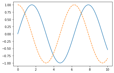
x = np.linspace(0, 10, 100)

fig = plt.figure()
plt.plot(x, np.sin(x), '-')
plt.plot(x, np.cos(x), '--');
#fig.savefig('my_figure.png')
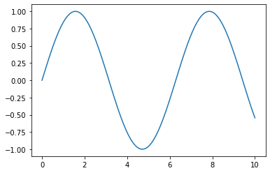
plt.plot(x, np.sin(x));
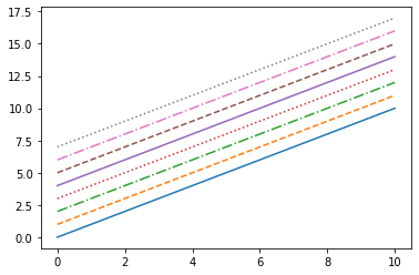
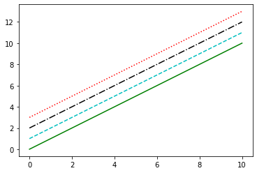
plt.plot(x, x + 0, linestyle='solid')
plt.plot(x, x + 1, linestyle='dashed')
plt.plot(x, x + 2, linestyle='dashdot')
plt.plot(x, x + 3, linestyle='dotted');

# For short, you can use the following codes:
plt.plot(x, x + 4, linestyle='-')  # solid
plt.plot(x, x + 5, linestyle='--') # dashed
plt.plot(x, x + 6, linestyle='-.') # dashdot
plt.plot(x, x + 7, linestyle=':');  # dotted
plt.plot(x, x + 0, '-g')  # solid green
plt.plot(x, x + 1, '--c') # dashed cyan
plt.plot(x, x + 2, '-.k') # dashdot black
plt.plot(x, x + 3, ':r');  # dotted red
plt.plot(x, np.sin(x), label="sin(x)")
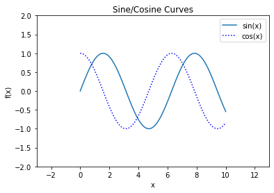
plt.plot(x, np.cos(x), ':b', label='cos(x)')

plt.xlim(-3, 13)
plt.ylim(-2, 2);
plt.title("Sine/Cosine Curves")
plt.xlabel("x")
plt.ylabel("f(x)");
plt.legend();
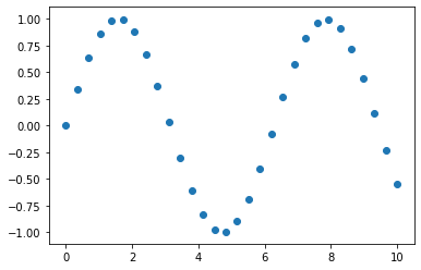
x = np.linspace(0, 10, 30)
y = np.sin(x)
plt.scatter(x, y, marker='o')
<matplotlib.collections.PathCollection at 0x7fdced88b550>
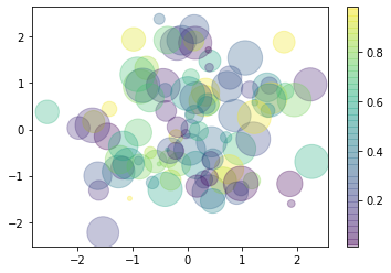
rng = np.random.RandomState(0)
x = rng.randn(100)
y = rng.randn(100)
colors = rng.rand(100)
sizes = 1000 * rng.rand(100)

plt.scatter(x, y, c=colors, s=sizes, alpha=0.3,
            cmap='viridis')
plt.colorbar();
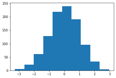
data = np.random.randn(1000)
plt.hist(data);
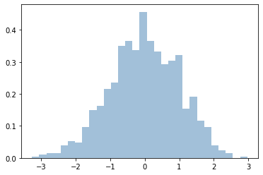
plt.hist(data, bins=30, density=True, alpha=0.5,
         histtype='stepfilled', color='steelblue',
         edgecolor='none');
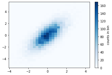
mean = [0, 0]
cov = [[1, 1], [1, 2]]
x, y = np.random.multivariate_normal(mean, cov, 10000).T
plt.hist2d(x, y, bins=30, cmap='Blues')
cb = plt.colorbar()
cb.set_label('counts in bin')
Multiple plots
MATLAB-style Interface
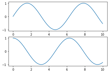
x = np.linspace(0, 10, 100)

plt.figure()  # create a plot figure

# create the first of two panels and set current axis
plt.subplot(2, 1, 1) # (rows, columns, panel number)
plt.plot(x, np.sin(x))

# create the second panel and set current axis
plt.subplot(2, 1, 2)
plt.plot(x, np.cos(x));

Object-oriented interface
# First create a grid of plots
# ax will be an array of two Axes objects
fig, ax = plt.subplots(2)

# Call plot() method on the appropriate object
ax[0].plot(x, np.sin(x))
ax[1].plot(x, np.cos(x));
Seaborn
https://seaborn.pydata.org/examples/index.html
import seaborn as sns
iris = sns.load_dataset("iris")
iris.head()
| sepal_length | sepal_width | petal_length | petal_width | species | |
|---|---|---|---|---|---|
| 0 | 5.1 | 3.5 | 1.4 | 0.2 | setosa |
| 1 | 4.9 | 3.0 | 1.4 | 0.2 | setosa |
| 2 | 4.7 | 3.2 | 1.3 | 0.2 | setosa |
| 3 | 4.6 | 3.1 | 1.5 | 0.2 | setosa |
| 4 | 5.0 | 3.6 | 1.4 | 0.2 | setosa |
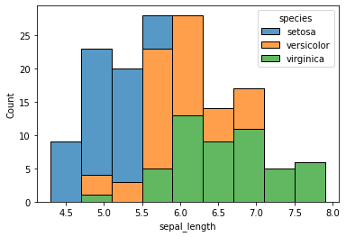
sns.histplot(data=iris, x="sepal_length", hue="species", multiple="stack");
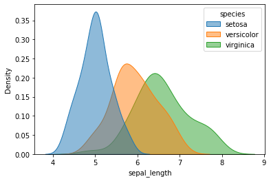
sns.kdeplot(data=iris, x="sepal_length", hue="species", shade=True, alpha=0.5);
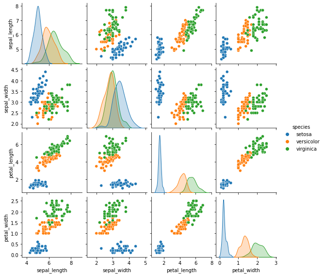
sns.pairplot(data=iris, hue='species', height=2);
